This post will review nonlinear covariation analysis developed by Müller & Sternad (2003). This purports to address several issues with UCM.
Movements are never exactly the same twice. There is noise in the system at all times and so any given execution will vary slightly from any other. the key insight of the motor abundance hypothesis is that there are multiple ways to do any task and so not all variability is equal. Only some of this variability will impact performance relative to a task goal; the rest will not stop you from achieving that goal. This insight is formalised in UCM and optimal control theory by only having motor control processes deployed to control the former variability. The latter is simply ignored (the manifold defining this subset of possible states is left 'uncontrolled').
This works because variability in one degree of freedom can be compensated for using another. If, as I reach for my coffee, my elbow begins to swing out my wrist and fingers can bend in the other direction so I still reach the cup. If this happens, the overall movement trajectory remains on the manifold and that elbow variation can be left alone. For Latash, this compensation is the signature of a synergy in action (in fact, it's his strict definition of a synergy).
Müller & Sternad note, however, that all this work has a problem. The covariation that occurs in a signature is often non-linear, and often involves more than two components. However, the tools deployed so far involve linear covariation analysis using linearised data, on pairs of components. Linearisation makes the data unsuitable for covariation analysis (it's no longer on an interval scale) while working with pairs limits the power of the techniques.
Their solution is a randomisation method to calculate covariation across multiple nonlinear relations. The basic form is this equation:
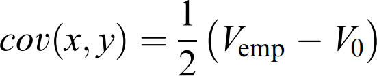
V(emp) is the variance you can measure empirically; V0 is the variance you'd expect if covariation was zero. Then then implement a slightly more generalised version but these two equations show the underlying structure of the analysis quite nicely. If you can get those numbers, you can compute the covariation between multiple nonlinearly related variables and quantify any synergies present in your data.
V(emp) is easy; you literally just compute the observed variance. But how can you possibly figure out V0?
Randomisation Methods
M&S then walk through a clear example to show how to estimate V0 using randomisation methods.

Imagine an arm who's job it is to land on a target at (20,40). There are three joint angles to worry about; α, β, and γ. M&S produced 10,000 normally distributed random angles for each joint, and found the 100 triplets that produced the most accurate landings. By definition, there should be some covariation going on here - the end result was success. You can now measure V(emp).
You can then estimate V0 by randomisation. Make a table with the triplets for the 100 successful reaches listed, and then randomly and independently mix the order of the columns for α, β, and γ. What you then have is three columns of data with most of the covariation removed, and it still has the same mean and variance of the true data set. Compute your measure of variance and that's what you'd expect with no covariation. They also repeat this process 100 times to get a sense of the distribution of the variance measure in randomised data sets, because of course a given randomisation might accidentally preserve or create some covariation of its own. The mean of this distribution is your final estimate of V0 and you can compute the covariation and test it for difference from 0. They then generalise this method and add a generalised correlation coefficient R.
Some Notes
- M&S demonstrate the randomisation on a subset of the trials. the best thing to do is do it on the whole data set, unless that set is so big the procedure begins to take ridiculous amounts of time, in which case a generous sample of the data can be used.
- You can assess variance using anything you like; standard deviations, or the bivariate variable error used in the example. All you need is a valid way to combine the data into a single measure.
- This procedure lets you not only compute all the necessary elements, but estimate your certainty about them too.
- I do not yet have any idea if this procedure can be applied to data prior to or as part of a UCM analysis or if that even makes sense. The authors don't do it, although this might just be because working to integrate methods is not something we're good at.
- If I get a chance I will implement their example in Matlab and post the code here. It was excellently clear!
Summary
This seems like quite a powerful method for measuring the presence of functionally significant covariation in a high dimensional, nonlinearly coupled movement data set. In other words, it will help you identify synergies. It does not seem to tell us much else, though; there's no identification of the manifold of goal equivalent states and so no way to quantify how much redundancy is present, etc. But, at this point, this analysis strikes me as a useful part of an overall toolbox and I look forward to getting into it in more detail.
References


Great summary Andrew! Adding some comments here (so that it does not seem like a Twitter rant)
ReplyDelete1. The TNC method "does" in fact identify the manifold of goal equivalent states. The function "f" that maps input to output variables is the "manifold" of equivalent solutions. The co-variation element is the equivalent of the "vucm/vort" metric in UCM. (generally true, but see reference below)
2. Regarding combining UCM and TNC - I'm not sure what the point would be unless it is for different aspects of a task. Because UCM is based on variance, it requires dimensionally similar elemental variables (either all forces, or all joint angles etc.) - there is no way to do a UCM analysis with dimensionally dissimilar variables like velocity and angle. The TNC gets around this issue by comparing the effects of variability at the "output" level.
Did you have anything specific in mind when you talked about combining them?
There is a nice paper comparing the two methods that detail some of the differences:
https://www.ncbi.nlm.nih.gov/pubmed/17715459
3. Finally, to complete the trio - there is also the GEM, where the biggest advance is that "time/trial order" is also now part of the analysis (both UCM and TNC at least in their original formulation are based only on variance - so trial order makes no difference). A good review of the GEM method is here:
https://www.ncbi.nlm.nih.gov/pubmed/24210574
Hope this helps - thanks again for doing this - your explanations are exceptionally clear! I'm going to refer my students to your blog from now on
Thanks for all your help finding these papers etc, I appreciate it! I'm really enjoying them all a lot and I'll take all the help I can get on figuring them out.
Delete1. Well then good, if that's in there that's great. I'm thinking of coding up their example to work through it some more, actually, so that might help.
2. re integrating this and UCM; I'm working on a project to test an idea I have for filling a gap in all these analyses, specifically formalising what the perceived task goal is. So I'm looking to apply my solution to all these 'motor abundance' analyses and develop a detailed analysis pipeline that can get applied by anyone else. If they don't specifically integrate, that's fine; complementary works too. But I don't see anyone working with all these analyses yet, it seems to have quickly devolved into camps.
re different dimensional variables; can you z transform the variance to get them on an equivalent scale? Or does that mess with something?
3. The Goal Equivalent Manifold is the last of my four motor abundance methods to review (thanks to you for all the references earlier on Twitter!)
Glad this is useful! Always happy to hear students will get something from this. And these are not my final thoughts, I'm still learning, so if I'm wrong or missing something let me know!
Hi Andrew
ReplyDeleteRe (2) - IMO, z-transforming variables actually takes away the value of these analyses because there is no longer a well-defined relation between the "task outcome variable" and the elemental variables - i.e., if I know the joint angles directly, I know where the end-point of the effector is, but if I only know the z-transformed joint angle, I probably have no way of estimating the position of the end-point. More conceptually, in the original framework having "more" or "less" variance in certain joint angles is meaningful because it directly relates to how much they contribute to the task (whereas the unit variance of the z-transform destroys that)
One sort of compromise is done in some of the UCM postural control papers, where they try to relate muscle activity to changes in the center-of-pressure. Here, there is no clear empirical relation between these two (unlike the joint angle vs end effector) - so they estimate this relation using a regression (assuming that deviations from the mean are small that they can be approximated by a matrix)
One last point - the UCM (at least in its original formulation) requires the input variables to be "elemental variables" - i.e. they at least in principle should be uncorrelated. This is why in force production studies because there is "enslaving" between the fingers (i.e. a force produced in one finger also causes small forces in other fingers), the elemental variables are no longer "finger forces" , but rather "finger modes" (which account for the fact that there is enslaving)
Thanks for all that! Very useful :)
Delete